[h=3]Probability mass function[/h]
In general, if the random variable K follows the binomial distribution with parameters n and p, we writeK ~ B(n, p). The probability of getting exactly k successes in n trials is given by the probability mass function:
<dl style="margin-top: 0.2em; margin-bottom: 0.5em; color: rgb(0, 0, 0); font-family: sans-serif; line-height: 19.1875px;"><dd style="line-height: 1.5em; margin-left: 1.6em; margin-bottom: 0.1em; margin-right: 0px;">
</dd></dl>
for k = 0, 1, 2, ..., n, where
<dl style="margin-top: 0.2em; margin-bottom: 0.5em; color: rgb(0, 0, 0); font-family: sans-serif; line-height: 19.1875px;"><dd style="line-height: 1.5em; margin-left: 1.6em; margin-bottom: 0.1em; margin-right: 0px;">
</dd></dl>
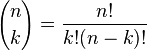
is the binomial coefficient (hence the name of the distribution) "n choose k", also denoted C(n, k), [SUB]n[/SUB]C[SUB]k[/SUB], or [SUP]n[/SUP]C[SUB]k[/SUB]. The formula can be understood as follows: we want k successes (p[SUP]k[/SUP]) and n − k failures (1 − p)[SUP]n − k[/SUP]. However, the k successes can occur anywhere among the n trials, and there are C(n, k) different ways of distributing k successes in a sequence of n trials.
In creating reference tables for binomial distribution probability, usually the table is filled in up to n/2 values. This is because for k > n/2, the probability can be calculated by its complement as
<dl style="margin-top: 0.2em; margin-bottom: 0.5em; color: rgb(0, 0, 0); font-family: sans-serif; line-height: 19.1875px;"><dd style="line-height: 1.5em; margin-left: 1.6em; margin-bottom: 0.1em; margin-right: 0px;">
</dd></dl>
Looking at the expression ƒ(k, n, p) as a function of k, there is a k value that maximizes it. This kvalue can be found by calculating
<dl style="margin-top: 0.2em; margin-bottom: 0.5em; color: rgb(0, 0, 0); font-family: sans-serif; line-height: 19.1875px;"><dd style="line-height: 1.5em; margin-left: 1.6em; margin-bottom: 0.1em; margin-right: 0px;">
</dd></dl>
and comparing it to 1. There is always an integer M that satisfies
<dl style="margin-top: 0.2em; margin-bottom: 0.5em; color: rgb(0, 0, 0); font-family: sans-serif; line-height: 19.1875px;"><dd style="line-height: 1.5em; margin-left: 1.6em; margin-bottom: 0.1em; margin-right: 0px;">
</dd></dl>
ƒ(k, n, p) is monotone increasing for k < M and monotone decreasing for k > M, with the exception of the case where (n + 1)p is an integer. In this case, there are two values for which ƒ is maximal: (n + 1)p and (n + 1)p − 1. M is the most probable (most likely) outcome of the Bernoulli trials and is called the mode. Note that the probability of it occurring can be fairly small.
[h=3][
edit]Cumulative distribution function[/h]
The cumulative distribution function can be expressed as:
<dl style="margin-top: 0.2em; margin-bottom: 0.5em; color: rgb(0, 0, 0); font-family: sans-serif; line-height: 19.1875px;"><dd style="line-height: 1.5em; margin-left: 1.6em; margin-bottom: 0.1em; margin-right: 0px;">
</dd></dl>
where
is the "floor" under x, i.e. the greatest integer less than or equal to x.
It can also be represented in terms of the regularized incomplete beta function, as follows:
<dl style="margin-top: 0.2em; margin-bottom: 0.5em; color: rgb(0, 0, 0); font-family: sans-serif; line-height: 19.1875px;"><dd style="line-height: 1.5em; margin-left: 1.6em; margin-bottom: 0.1em; margin-right: 0px;">
</dd></dl>
For k ≤ np, upper bounds for the lower tail of the distribution function can be derived. In particular,Hoeffding's inequality yields the bound
<dl style="margin-top: 0.2em; margin-bottom: 0.5em; color: rgb(0, 0, 0); font-family: sans-serif; line-height: 19.1875px;"><dd style="line-height: 1.5em; margin-left: 1.6em; margin-bottom: 0.1em; margin-right: 0px;">
</dd></dl>
and Chernoff's inequality can be used to derive the bound
<dl style="margin-top: 0.2em; margin-bottom: 0.5em; color: rgb(0, 0, 0); font-family: sans-serif; line-height: 19.1875px;"><dd style="line-height: 1.5em; margin-left: 1.6em; margin-bottom: 0.1em; margin-right: 0px;">
</dd></dl>
Moreover, these bounds are reasonably tight when p = 1/2, since the following expression holds for all k ≥ 3n/8[SUP][1][/SUP]
<dl style="margin-top: 0.2em; margin-bottom: 0.5em; color: rgb(0, 0, 0); font-family: sans-serif; line-height: 19.1875px;"><dd style="line-height: 1.5em; margin-left: 1.6em; margin-bottom: 0.1em; margin-right: 0px;">
</dd></dl>[h=2][
edit]Example[/h]
Suppose a biased coin comes up heads with probability 0.3 when tossed. What is the probability of achieving 0, 1,..., 6 heads after six tosses?
<dl style="margin-top: 0.2em; margin-bottom: 0.5em; color: rgb(0, 0, 0); font-family: sans-serif; line-height: 19.1875px;"><dd style="line-height: 1.5em; margin-left: 1.6em; margin-bottom: 0.1em; margin-right: 0px;">
</dd></dl><dl style="margin-top: 0.2em; margin-bottom: 0.5em; color: rgb(0, 0, 0); font-family: sans-serif; line-height: 19.1875px;"><dd style="line-height: 1.5em; margin-left: 1.6em; margin-bottom: 0.1em; margin-right: 0px;">
</dd></dl><dl style="margin-top: 0.2em; margin-bottom: 0.5em; color: rgb(0, 0, 0); font-family: sans-serif; line-height: 19.1875px;"><dd style="line-height: 1.5em; margin-left: 1.6em; margin-bottom: 0.1em; margin-right: 0px;">
</dd></dl><dl style="margin-top: 0.2em; margin-bottom: 0.5em; color: rgb(0, 0, 0); font-family: sans-serif; line-height: 19.1875px;"><dd style="line-height: 1.5em; margin-left: 1.6em; margin-bottom: 0.1em; margin-right: 0px;">
</dd></dl><dl style="margin-top: 0.2em; margin-bottom: 0.5em; color: rgb(0, 0, 0); font-family: sans-serif; line-height: 19.1875px;"><dd style="line-height: 1.5em; margin-left: 1.6em; margin-bottom: 0.1em; margin-right: 0px;">
</dd></dl><dl style="margin-top: 0.2em; margin-bottom: 0.5em; color: rgb(0, 0, 0); font-family: sans-serif; line-height: 19.1875px;"><dd style="line-height: 1.5em; margin-left: 1.6em; margin-bottom: 0.1em; margin-right: 0px;">
</dd></dl><dl style="margin-top: 0.2em; margin-bottom: 0.5em; color: rgb(0, 0, 0); font-family: sans-serif; line-height: 19.1875px;"><dd style="line-height: 1.5em; margin-left: 1.6em; margin-bottom: 0.1em; margin-right: 0px;">
[SUP]
[2][/SUP]</dd></dl>[h=2][
edit]Mean and variance[/h]
If X ~ B(n, p) (that is, X is a binomially distributed random variable), then the expected value of X is
<dl style="margin-top: 0.2em; margin-bottom: 0.5em; color: rgb(0, 0, 0); font-family: sans-serif; line-height: 19.1875px;"><dd style="line-height: 1.5em; margin-left: 1.6em; margin-bottom: 0.1em; margin-right: 0px;">
</dd></dl>
and the variance is
<dl style="margin-top: 0.2em; margin-bottom: 0.5em; color: rgb(0, 0, 0); font-family: sans-serif; line-height: 19.1875px;"><dd style="line-height: 1.5em; margin-left: 1.6em; margin-bottom: 0.1em; margin-right: 0px;">
</dd></dl>[h=2][
edit]Mode and median[/h]
Usually the mode of a binomial B(n, p) distribution is equal to
, where
is the floor function. However when (n + 1)p is an integer and p is neither 0 nor 1, then the distribution has two modes: (n + 1)p and (n + 1)p − 1. When p is equal to 0 or 1, the mode will be 0 and n correspondingly. These cases can be summarized as follows:
<dl style="margin-top: 0.2em; margin-bottom: 0.5em; color: rgb(0, 0, 0); font-family: sans-serif; line-height: 19.1875px;"><dd style="line-height: 1.5em; margin-left: 1.6em; margin-bottom: 0.1em; margin-right: 0px;">
</dd></dl>
In general, there is no single formula to find the median for a binomial distribution, and it may even be non-unique. However several special results have been established:
- If np is an integer, then the mean, median, and mode coincide and equal np.[SUP][3][/SUP][SUP][4][/SUP]
- Any median m must lie within the interval ⌊np⌋ ≤ m ≤ ⌈np⌉.[SUP][5][/SUP]
- A median m cannot lie too far away from the mean: |m − np| ≤ min{ ln 2, max{p, 1 − p} }.[SUP][6][/SUP]
- The median is unique and equal to m = round(np) in cases when either p ≤ 1 − ln 2 or p ≥ ln 2 or |m − np| ≤ min{p, 1 − p} (except for the case when p = ½ and nis odd).[SUP][5][/SUP][SUP][6][/SUP]
- When p = 1/2 and n is odd, any number m in the interval ½(n − 1) ≤ m ≤ ½(n + 1) is a median of the binomial distribution. If p = 1/2 and n is even, then m = n/2 is the unique median.
[h=2][
edit]Covariance between two binomials[/h]
If two binomially distributed random variables X and Y are observed together, estimating their covariance can be useful. Using the definition of covariance, in the casen = 1 (thus being Bernoulli trials) we have
<dl style="margin-top: 0.2em; margin-bottom: 0.5em; color: rgb(0, 0, 0); font-family: sans-serif; line-height: 19.1875px;"><dd style="line-height: 1.5em; margin-left: 1.6em; margin-bottom: 0.1em; margin-right: 0px;">
</dd></dl>
The first term is non-zero only when both X and Y are one, and μ[SUB]X[/SUB] and μ[SUB]Y[/SUB] are equal to the two probabilities. Defining p[SUB]B[/SUB] as the probability of both happening at the same time, this gives
<dl style="margin-top: 0.2em; margin-bottom: 0.5em; color: rgb(0, 0, 0); font-family: sans-serif; line-height: 19.1875px;"><dd style="line-height: 1.5em; margin-left: 1.6em; margin-bottom: 0.1em; margin-right: 0px;">
</dd></dl>
and for n such trials again due to independence
<dl style="margin-top: 0.2em; margin-bottom: 0.5em; color: rgb(0, 0, 0); font-family: sans-serif; line-height: 19.1875px;"><dd style="line-height: 1.5em; margin-left: 1.6em; margin-bottom: 0.1em; margin-right: 0px;">
</dd></dl>
If X and Y are the same variable, this reduces to the variance formula given above.
[h=2][
edit]Relationship to other distributions[/h][h=3][
edit]Sums of binomials[/h]
If X ~ B(n, p) and Y ~ B(m, p) are independent binomial variables with the same probability p, then X + Y is again a binomial variable; its distribution is[SUP][citation needed][/SUP]
<dl style="margin-top: 0.2em; margin-bottom: 0.5em; color: rgb(0, 0, 0); font-family: sans-serif; line-height: 19.1875px;"><dd style="line-height: 1.5em; margin-left: 1.6em; margin-bottom: 0.1em; margin-right: 0px;">
</dd></dl>[h=3][
edit]Conditional binomials[/h]
If X ~ B(n, p) and, conditional on X, Y ~ B(X, q), then Y is a simple binomial variable with distribution[SUP][citation needed][/SUP]
<dl style="margin-top: 0.2em; margin-bottom: 0.5em; color: rgb(0, 0, 0); font-family: sans-serif; line-height: 19.1875px;"><dd style="line-height: 1.5em; margin-left: 1.6em; margin-bottom: 0.1em; margin-right: 0px;">
</dd></dl>[h=3][
edit]Bernoulli distribution[/h]
The Bernoulli distribution is a special case of the binomial distribution, where n = 1. Symbolically, X ~ B(1, p) has the same meaning as X ~ Bern(p). Conversely, any binomial distribution, B(n, p), is the sum of n independent Bernoulli trials, Bern(p), each with the same probability p.[SUP][citation needed][/SUP]
[h=3][
edit]Poisson binomial distribution[/h]
The binomial distribution is a special case of the Poisson binomial distribution, which is a sum of n independent non-identical Bernoulli trials Bern(p[SUB]i[/SUB]).[SUP][citation needed][/SUP]If X has the Poisson binomial distribution with p[SUB]1[/SUB] = … = p[SUB]n[/SUB] =p then X ~ B(n, p).
[h=3][
edit]Normal approximation[/h]


Binomial PDF and normal approximation for
n = 6 and
p = 0.5
If n is large enough, then the skew of the distribution is not too great. In this case a reasonable approximation to B(n, p) is given by the normal distribution
<dl style="margin-top: 0.2em; margin-bottom: 0.5em; color: rgb(0, 0, 0); font-family: sans-serif; line-height: 19.1875px;"><dd style="line-height: 1.5em; margin-left: 1.6em; margin-bottom: 0.1em; margin-right: 0px;">
</dd></dl>
and this basic approximation can be improved in a simple way by using a suitable continuity correction. The basic approximation generally improves as n increases (at least 20) and is better when p is not near to 0 or 1.[SUP][7][/SUP] Variousrules of thumb may be used to decide whether n is large enough, and p is far enough from the extremes of zero or one:
- One rule is that both x=np and n(1 − p) must be greater than 5. However, the specific number varies from source to source, and depends on how good an approximation one wants; some sources give 10 which gives virtually the same results as the following rule for large n until n is very large (ex: x=11, n=7752).
- A second rule[SUP][7][/SUP] is that for n > 5 the normal approximation is adequate if
<dl style="margin-top: 0.2em; margin-bottom: 0.5em; color: rgb(0, 0, 0); font-family: sans-serif; line-height: 19.1875px;"><dd style="line-height: 1.5em; margin-left: 1.6em; margin-bottom: 0.1em; margin-right: 0px;"><dl style="margin-top: 0.2em; margin-bottom: 0.5em;"><dd style="line-height: 1.5em; margin-left: 1.6em; margin-bottom: 0.1em; margin-right: 0px;">
</dd></dl></dd></dl>
- Another commonly used rule holds that the normal approximation is appropriate only if everything within 3 standard deviations of its mean is within the range of possible values,[SUP][citation needed][/SUP] that is if
<dl style="margin-top: 0.2em; margin-bottom: 0.5em; color: rgb(0, 0, 0); font-family: sans-serif; line-height: 19.1875px;"><dd style="line-height: 1.5em; margin-left: 1.6em; margin-bottom: 0.1em; margin-right: 0px;"><dl style="margin-top: 0.2em; margin-bottom: 0.5em;"><dd style="line-height: 1.5em; margin-left: 1.6em; margin-bottom: 0.1em; margin-right: 0px;">
</dd></dl></dd></dl>
The following is an example of applying a continuity correction. Suppose one wishes to calculate Pr(X ≤ 8) for a binomial random variable X. If Y has a distribution given by the normal approximation, then Pr(X ≤ 8) is approximated by Pr(Y ≤ 8.5). The addition of 0.5 is the continuity correction; the uncorrected normal approximation gives considerably less accurate results.
This approximation, known as de Moivre–Laplace theorem, is a huge time-saver when undertaking calculations by hand (exact calculations with large n are very onerous); historically, it was the first use of the normal distribution, introduced in Abraham de Moivre's book The Doctrine of Chances in 1738. Nowadays, it can be seen as a consequence of the central limit theorem since B(n, p) is a sum of n independent, identically distributed Bernoulli variables with parameter p. This fact is the basis of a hypothesis test, a "proportion z-test," for the value of p using x/n, the sample proportion and estimator of p, in a common test statistic.[SUP][8][/SUP]
For example, suppose one randomly samples n people out of a large population and ask them whether they agree with a certain statement. The proportion of people who agree will of course depend on the sample. If groups of n people were sampled repeatedly and truly randomly, the proportions would follow an approximate normal distribution with mean equal to the true proportion p of agreement in the population and with standard deviation σ = (p(1 − p)/n)[SUP]1/2[/SUP]. Large sample sizes n are good because the standard deviation, as a proportion of the expected value, gets smaller, which allows a more precise estimate of the unknown parameter p.
[h=3][
edit]Poisson approximation[/h]
The binomial distribution converges towards the Poisson distribution as the number of trials goes to infinity while the product np remains fixed. Therefore the Poisson distribution with parameter λ = np can be used as an approximation to B(n, p) of the binomial distribution if n is sufficiently large and p is sufficiently small. According to two rules of thumb, this approximation is good if n ≥ 20 and p ≤ 0.05, or if n ≥ 100 and np ≤ 10.[SUP][9][/SUP]
[h=3][
edit]Limiting distributions[/h]
<dl style="margin-top: 0.2em; margin-bottom: 0.5em; color: rgb(0, 0, 0); font-family: sans-serif; line-height: 19.1875px;"><dd style="line-height: 1.5em; margin-left: 1.6em; margin-bottom: 0.1em; margin-right: 0px;"><dl style="margin-top: 0.2em; margin-bottom: 0.5em;"><dd style="line-height: 1.5em; margin-left: 1.6em; margin-bottom: 0.1em; margin-right: 0px;">
</dd></dl></dd></dl><dl style="margin-top: 0.2em; margin-bottom: 0.5em; color: rgb(0, 0, 0); font-family: sans-serif; line-height: 19.1875px;"><dd style="line-height: 1.5em; margin-left: 1.6em; margin-bottom: 0.1em; margin-right: 0px;">approaches the
normal distribution with expected value 0 and
variance 1.[SUP][
citation needed][/SUP] This result is sometimes loosely stated by saying that the distribution of
X is
asymptotically normal with expected value
np and
variance np(1 −
p). This result is a specific case of the
central limit theorem.</dd></dl>[h=2][
edit]Confidence intervals[/h]
Main article: Binomial proportion confidence interval
Even for quite large values of n, the actual distribution of the mean is significantly nonnormal.[SUP][10][/SUP] Because of this problem several methods to estimate confidence intervals have been proposed.
Let n[SUB]1[/SUB] be the number of successes out of n, the total number of trials, and let
<dl style="margin-top: 0.2em; margin-bottom: 0.5em; color: rgb(0, 0, 0); font-family: sans-serif; line-height: 19.1875px;"><dd style="line-height: 1.5em; margin-left: 1.6em; margin-bottom: 0.1em; margin-right: 0px;">
</dd></dl>
be the proportion of successes. Let z[SUB]α/2[/SUB] be the 100 ( 1 − α / 2 )[SUP]th[/SUP] percentile of the standard normal distribution.
<dl style="margin-top: 0.2em; margin-bottom: 0.5em; color: rgb(0, 0, 0); font-family: sans-serif; line-height: 19.1875px;"><dd style="line-height: 1.5em; margin-left: 1.6em; margin-bottom: 0.1em; margin-right: 0px;">
</dd></dl>
A continuity correction of 0.5/n may be added.[SUP][clarification needed][/SUP]
- Agresti-Coull method[SUP][11][/SUP]
<dl style="margin-top: 0.2em; margin-bottom: 0.5em; color: rgb(0, 0, 0); font-family: sans-serif; line-height: 19.1875px;"><dd style="line-height: 1.5em; margin-left: 1.6em; margin-bottom: 0.1em; margin-right: 0px;">
</dd></dl>
Here the estimate of p is modified to
<dl style="margin-top: 0.2em; margin-bottom: 0.5em; color: rgb(0, 0, 0); font-family: sans-serif; line-height: 19.1875px;"><dd style="line-height: 1.5em; margin-left: 1.6em; margin-bottom: 0.1em; margin-right: 0px;">
</dd></dl>
- ArcSine method[SUP][12][/SUP]
<dl style="margin-top: 0.2em; margin-bottom: 0.5em; color: rgb(0, 0, 0); font-family: sans-serif; line-height: 19.1875px;"><dd style="line-height: 1.5em; margin-left: 1.6em; margin-bottom: 0.1em; margin-right: 0px;">
</dd></dl>
- Wilson (score) method[SUP][13][/SUP]
<dl style="margin-top: 0.2em; margin-bottom: 0.5em; color: rgb(0, 0, 0); font-family: sans-serif; line-height: 19.1875px;"><dd style="line-height: 1.5em; margin-left: 1.6em; margin-bottom: 0.1em; margin-right: 0px;">
</dd></dl>